TrajNet++
TrajNet++ is a pedestrian forecasting challenge [KKA21]. This notebook walks through a first attempt to fit to real-world data from this challenge [LCL07].
Synthetic Data
circle = socialforce.scenarios.Circle()
synthetic_scenarios = circle.generate(1)
synthetic_experience = socialforce.Trainer.scenes_to_experience(synthetic_scenarios)
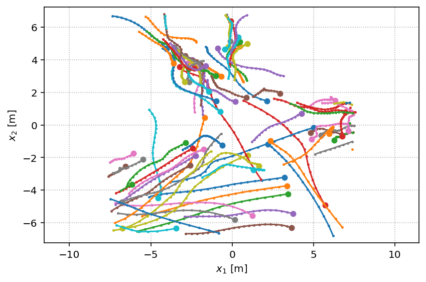
with socialforce.show.track_canvas() as ax:
socialforce.show.states(ax, synthetic_scenarios[0])
!ls ../data-trajnet/train/real_data/
trajnet_scenes = list(socialforce.trajnet.Reader('../data-trajnet/train/real_data/crowds_students001.ndjson').scenes())[:2]
biwi_hotel.ndjson  cff_13.ndjson	      crowds_students003.ndjson
cff_06.ndjson	   cff_14.ndjson	      crowds_zara01.ndjson
cff_07.ndjson	   cff_15.ndjson	      crowds_zara03.ndjson
cff_08.ndjson	   cff_16.ndjson	      lcas.ndjson
cff_09.ndjson	   cff_17.ndjson	      wildtrack.ndjson
cff_10.ndjson	   cff_18.ndjson
cff_12.ndjson	   crowds_students001.ndjson
V = socialforce.potentials.PedPedPotentialMLP()
initial_state_dict = copy.deepcopy(V.state_dict())

simulator = socialforce.Simulator(ped_ped=V)
def trajnet_to_socialforce_scenario(pxy):
pxy = torch.from_numpy(pxy)
velocities = (pxy[1:] - pxy[:-1]) * 2.5 # convert to m/s with FPS
states = torch.full((pxy.shape[0], pxy.shape[1], 4), float('nan'))
states[:, :, :2] = pxy
states[:-1, :, 2:4] = velocities
states[-1, :, 2:4] = velocities[-1]
return torch.stack([simulator.normalize_state(state) for state in states], dim=0)
scenarios = [
trajnet_to_socialforce_scenario(pxy)
for _, pxy in trajnet_scenes
]
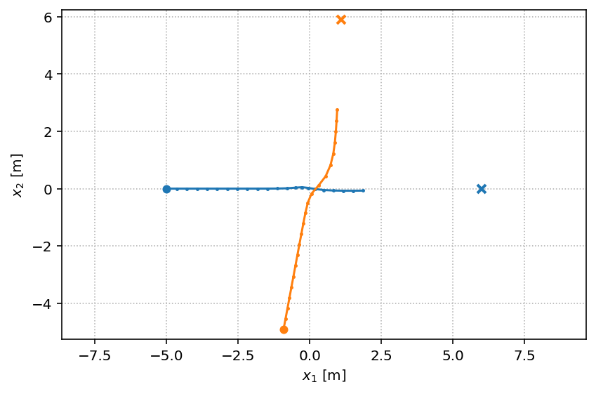
with socialforce.show.track_canvas() as ax:
socialforce.show.states(ax, scenarios[0])
true_experience = socialforce.Trainer.scenes_to_experience(scenarios)
print(true_experience[0][0][0], true_experience[0][1][0])
tensor([ 3.2100, -3.2100, -1.1250, -0.1750,  0.0000,  0.0000,     nan,     nan,
         0.5000,  1.1385]) tensor([ 2.7600, -3.2800, -1.1500, -0.1500,  0.0000,  0.0000,     nan,     nan,
         0.5000,  1.1597])
MLP
We infer the parameters of an MLP to approximate the 1D scalar
function \(\textrm{SF}(b)\) above from synthetic observations.
The PedPedPotentialMLP is a two-layer MLP with softplus activations:
which is written in terms of linear and non-linear operators where the Softplus operator applies the softplus function on its input from the right and \(L\) is a linear operator (a matrix) with the subscript indicating the \(\textrm{output features} \times \textrm{input features}\). This two-layer MLP with 5 hidden units has 10 parameters.
# moved up
Inference
We use a standard optimizer from PyTorch (SGD).
You can specify a standard PyTorch loss function for the Trainer as well
but here the default of a torch.nn.L1Loss() is used.
# HIDE OUTPUT
# moved up simulator = socialforce.Simulator(ped_ped=V)
opt = torch.optim.SGD(V.parameters(), lr=1.0)
socialforce.Trainer(simulator, opt).loop(100, synthetic_experience, log_interval=10)
synthetic_state_dict = copy.deepcopy(V.state_dict())
epoch 10: 0.012627490679733455
epoch 20: 0.010980502236634493
epoch 30: 0.00995746738044545
epoch 40: 0.008148402615915984
epoch 50: 0.004848372656852007
epoch 60: 0.0021347774018067867
epoch 70: 0.0009875366813503206
epoch 80: 0.0016503104416187853
epoch 90: 0.001486208027927205
epoch 100: 0.0007074080058373511
opt = torch.optim.SGD(V.parameters(), lr=0.1)
loss = torch.nn.SmoothL1Loss(beta=0.1)
socialforce.Trainer(simulator, opt, loss=loss).loop(10, true_experience)
final_state_dict = copy.deepcopy(V.state_dict())
epoch 1: 0.010607893299311399
epoch 2: 0.007377330691087991
epoch 3: 0.00533741976832971
epoch 4: 0.0040055212448351085
epoch 5: 0.0031346069765277205
epoch 6: 0.0025307023606728762
epoch 7: 0.002101081085857004
epoch 8: 0.001783407453331165
epoch 9: 0.001538612542208284
epoch 10: 0.0013477462402079255
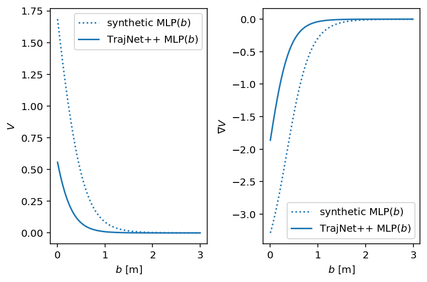
# HIDE CODE
with socialforce.show.canvas(ncols=2) as (ax1, ax2):
    # V.load_state_dict(initial_state_dict)
    # socialforce.show.potential_1d(V, ax1, ax2, label=r'initial MLP($b$)', linestyle='dashed', color='C0')

    V.load_state_dict(synthetic_state_dict)
    socialforce.show.potential_1d(V, ax1, ax2, label=r'synthetic MLP($b$)', linestyle='dotted', color='C0')

    V.load_state_dict(final_state_dict)
    socialforce.show.potential_1d(V, ax1, ax2, label=r'TrajNet++ MLP($b$)', color='C0')