1D Wall
Parametric
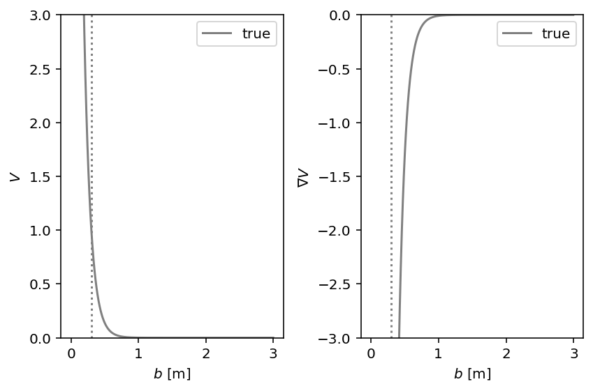
This is an extension of the 1D example to study the robustness of the inference process to potentials with steep gradients. We use a modified \(V(b)\) potential that could be described as a “soft wall” at \(b=\sigma\). The amount of gradients is determined by the width \(w\) of this wall:
with its two parameters \(\sigma\) and \(w\).
ped_ped = socialforce.potentials.PedPedPotentialWall(w=0.1)
with socialforce.show.canvas(ncols=2) as (ax1, ax2):
    ax1.set_ylim(0.0, 3.0)
    ax2.set_ylim(-3.0, 0.0)
    socialforce.show.potential_1d_parametric(
        ped_ped, ax1, ax2,
        label=r'true', sigma_label=r'true $\sigma$', color='gray')
Scenario
We generate a single Circle scenario.
circle = socialforce.scenarios.Circle(ped_ped=ped_ped)
scenario = circle.generate(1)
true_experience = socialforce.Trainer.scenes_to_experience(scenario)

with socialforce.show.track_canvas() as ax:
    socialforce.show.states(ax, scenario[0])
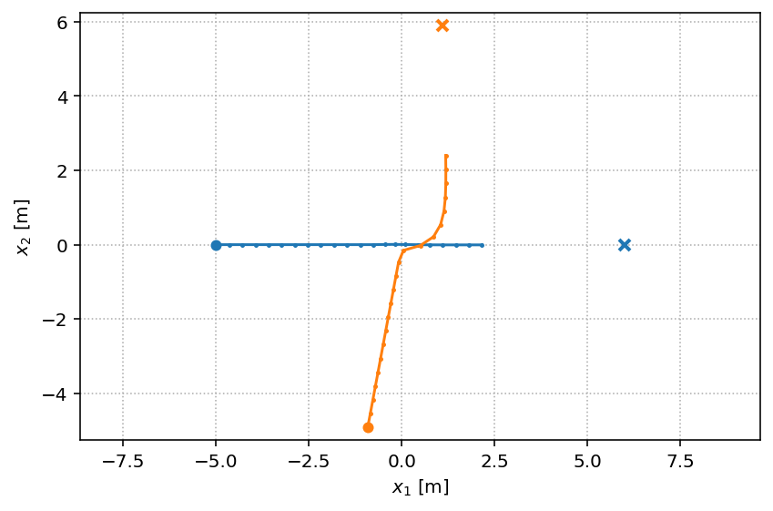
This synthetic path shows a non-smooth direction change of the orange pedestrian. This is an artifact stemming from the finite step size in the simulation of the dynamics. We could remove this artifact by increasing the oversampling in our simulation.
MLP
We infer the parameters of an MLP to approximate the 1D scalar
function \(\textrm{SF}(b)\) above from synthetic observations.
The PedPedPotentialMLP is a two-layer MLP with softplus activations:
which is written in terms of linear and non-linear operators where the Softplus operator applies the softplus function on its input from the right and \(L\) is a linear operator (a matrix) with the subscript indicating the \(\textrm{output features} \times \textrm{input features}\). This two-layer MLP with 5 hidden units has 10 parameters.
V = socialforce.potentials.PedPedPotentialMLP(hidden_units=8)
initial_state_dict = copy.deepcopy(V.state_dict())
Inference
We use a standard optimizer from PyTorch (SGD).
You can specify a standard PyTorch loss function for the Trainer as well
but here the default of a torch.nn.L1Loss() is used.
simulator = socialforce.Simulator(ped_ped=V)
opt = torch.optim.SGD(V.parameters(), lr=3.0)
socialforce.Trainer(simulator, opt).loop(100, true_experience, log_interval=10)
final_state_dict = copy.deepcopy(V.state_dict())
epoch 10: 0.01935910070980234
epoch 20: 0.01923418208025396
epoch 30: 0.019103735252948745
epoch 40: 0.018915292507569705
epoch 50: 0.01855790857890887
epoch 60: 0.017838151094370654
epoch 70: 0.017187436377363547
epoch 80: 0.01637901269298579
epoch 90: 0.01500139628270907
epoch 100: 0.012028532202488609
# HIDE CODE
with socialforce.show.canvas(ncols=2) as (ax1, ax2):
    ax1.set_ylim(0.0, 3.0)
    ax2.set_ylim(-3.0, 0.0)

    socialforce.show.potential_1d_parametric(
        circle.ped_ped, ax1, ax2,
        label=r'true $V_0 e^{-b/\sigma}$', sigma_label=r'true $\sigma$', color='gray')

    V.load_state_dict(initial_state_dict)
    socialforce.show.potential_1d(V, ax1, ax2, label=r'initial MLP($b$)', linestyle='dashed', color='C0')

    V.load_state_dict(final_state_dict)
    socialforce.show.potential_1d(V, ax1, ax2, label=r'MLP($b$)', color='C0')
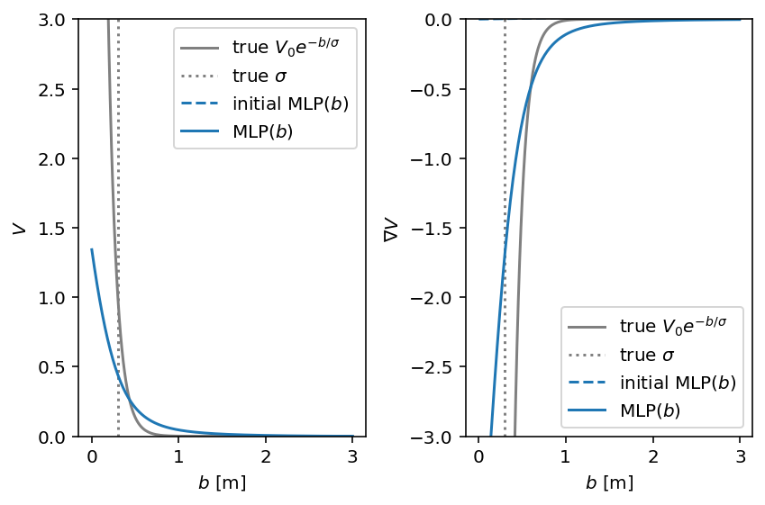
We can see that the numerical challenges impact our ability to infer the parameters of this potential. When we reduce \(w\) further, this discrepancy grows.