Diamond¶

Parametric¶

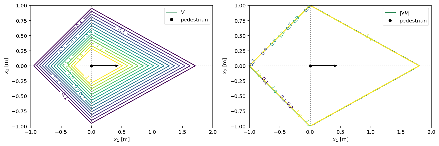
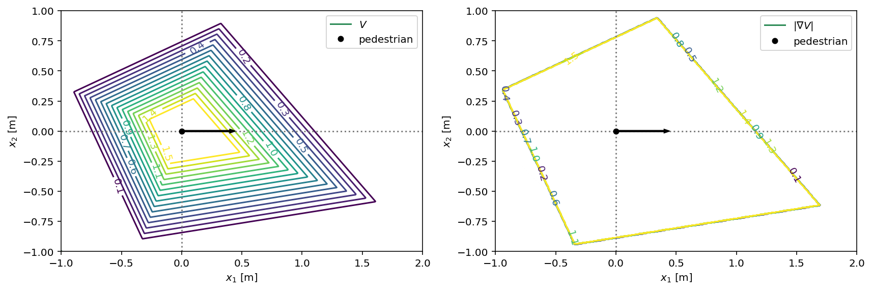
This is an extension of the 2D example to study the robustness of the inference process to potentials with gradients that change orientation. We use a modified \(V(b)\) potential that could be described as a “diamond” of height \(V_0\) and with a half-width of \(\sigma\):

(12)¶\[\begin{align} V(b) &= V_0 \max\left(0, 1 - \frac{|x_1| + |x_2|}{2\sigma} \right) \end{align}\]

with its two parameters \(V_0\) and \(\sigma\).

socialforce.FieldOfView.out_of_view_factor = 0.0

V = socialforce.potentials.PedPedPotentialDiamond(sigma=0.5)
with socialforce.show.canvas(figsize=(12, 6), ncols=2) as (ax1, ax2):
    socialforce.show.potential_2d(V, ax1)
    socialforce.show.potential_2d_grad(V, ax2)

Scenarios¶

Now we use the above parametric potential in a simulation to generate synthetic scenarios according to this potential. We generate Circle and ParallelOvertake scenarios.

circle = socialforce.scenarios.Circle(ped_ped=V)
parallel_overtake = socialforce.scenarios.ParallelOvertake(ped_ped=V)
parallel_avoidance = socialforce.scenarios.ParallelAvoidance(ped_ped=V)
scenarios = circle.generate(50) + parallel_overtake.generate(50) + parallel_avoidance.generate(150)
true_experience = socialforce.Trainer.scenes_to_experience(scenarios)

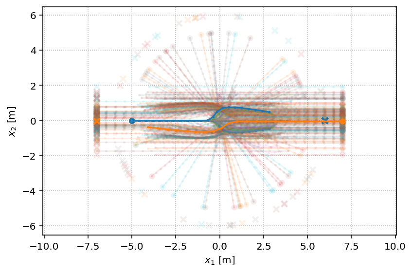
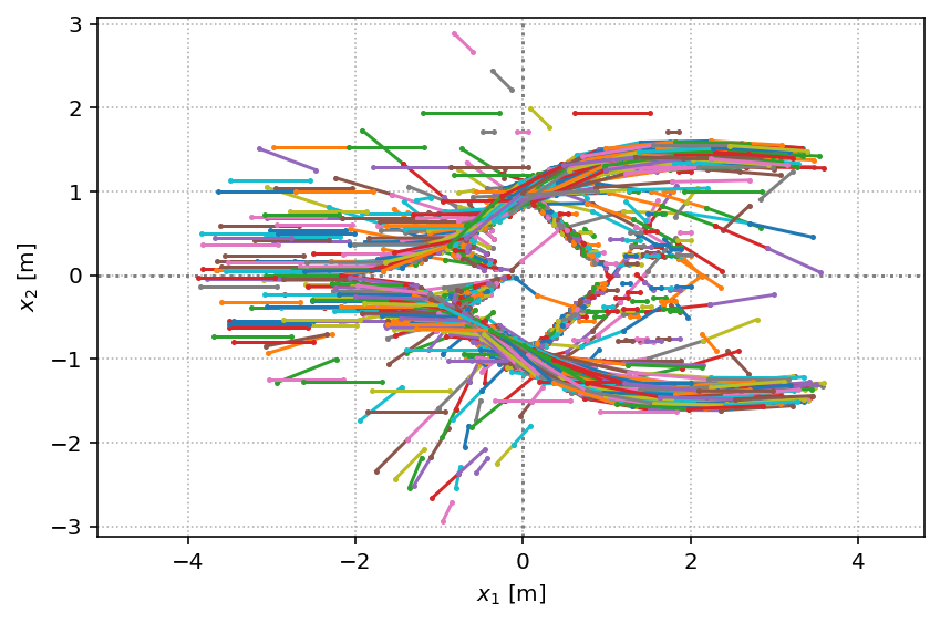
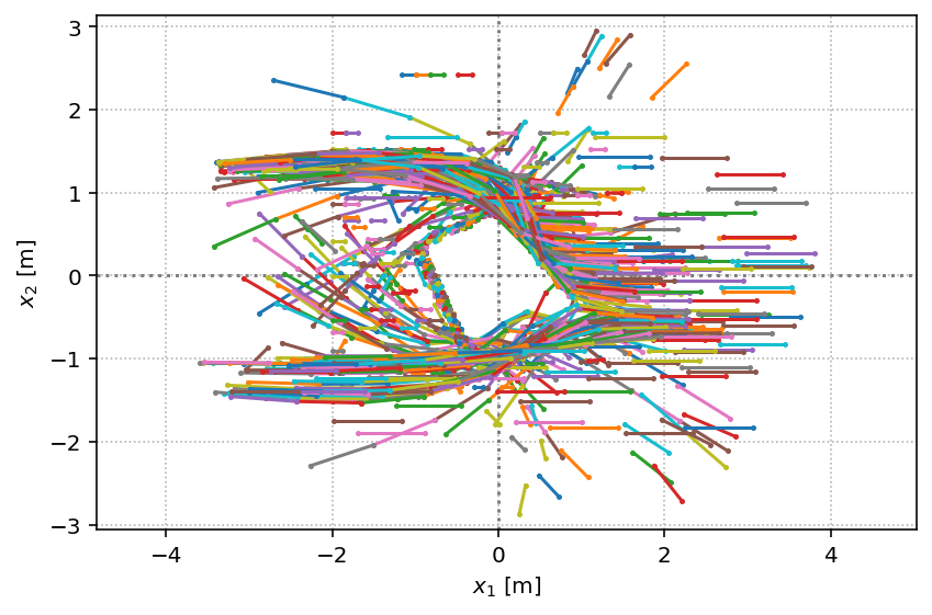
All the scenes from a fixed observer:

# HIDE CODE
with socialforce.show.track_canvas() as ax:
    socialforce.show.states(ax, scenarios[-1], zorder=10)
    for scene in scenarios[:-1]:
        socialforce.show.states(ax, scene, alpha=0.1)

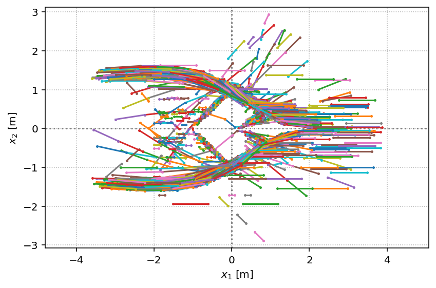
Parallel Overtake and Avoidance scenes from the perspective of the primary pedestrian:

# HIDE CODE
with socialforce.show.track_canvas() as ax:
    socialforce.show.experience(ax, true_experience)

From the perspective of the other pedestrian:

# HIDE CELL
with socialforce.show.track_canvas() as ax:
    socialforce.show.experience(ax, true_experience, reference_ped=1)

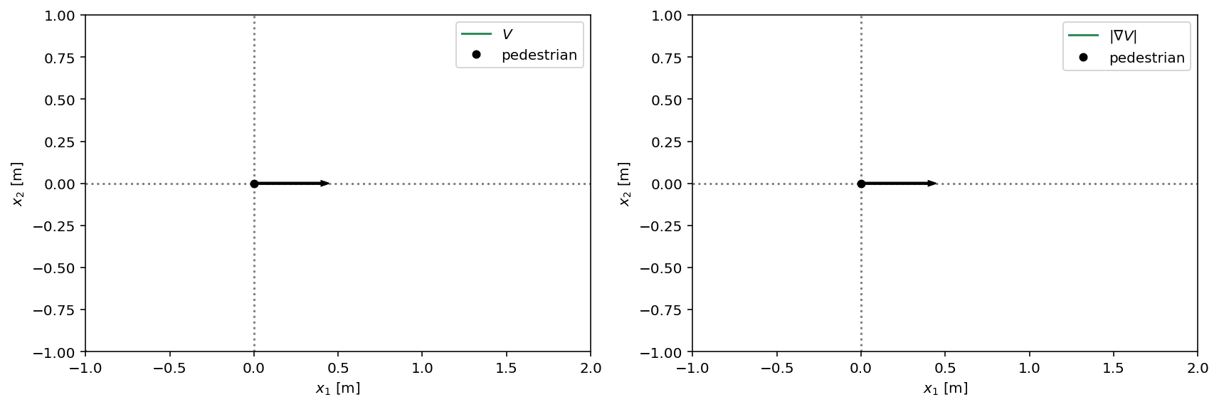
MLP Inference¶

We construct an coordinate-based MLP with Fourier Features [RR+07, TSM+20].

V = socialforce.potentials.PedPedPotentialMLP2D(hidden_units=32, n_hidden_layers=3)
with socialforce.show.canvas(figsize=(12, 6), ncols=2) as (ax1, ax2):
    socialforce.show.potential_2d(V, ax1)
    socialforce.show.potential_2d_grad(V, ax2)

/home/runner/work/socialforce/socialforce/socialforce/show.py:253: UserWarning: No contour levels were found within the data range.
  ax.contour(x1, x2, values.T,

simulator = socialforce.Simulator(ped_ped=V)
opt = torch.optim.SGD(V.parameters(), lr=0.03, momentum=0.9, nesterov=True)
# socialforce.Trainer(simulator, opt).loop(10, true_experience)  # does not work

with socialforce.show.canvas(figsize=(12, 6), ncols=2) as (ax1, ax2):
    socialforce.show.potential_2d(V, ax1)
    socialforce.show.potential_2d_grad(V, ax2)

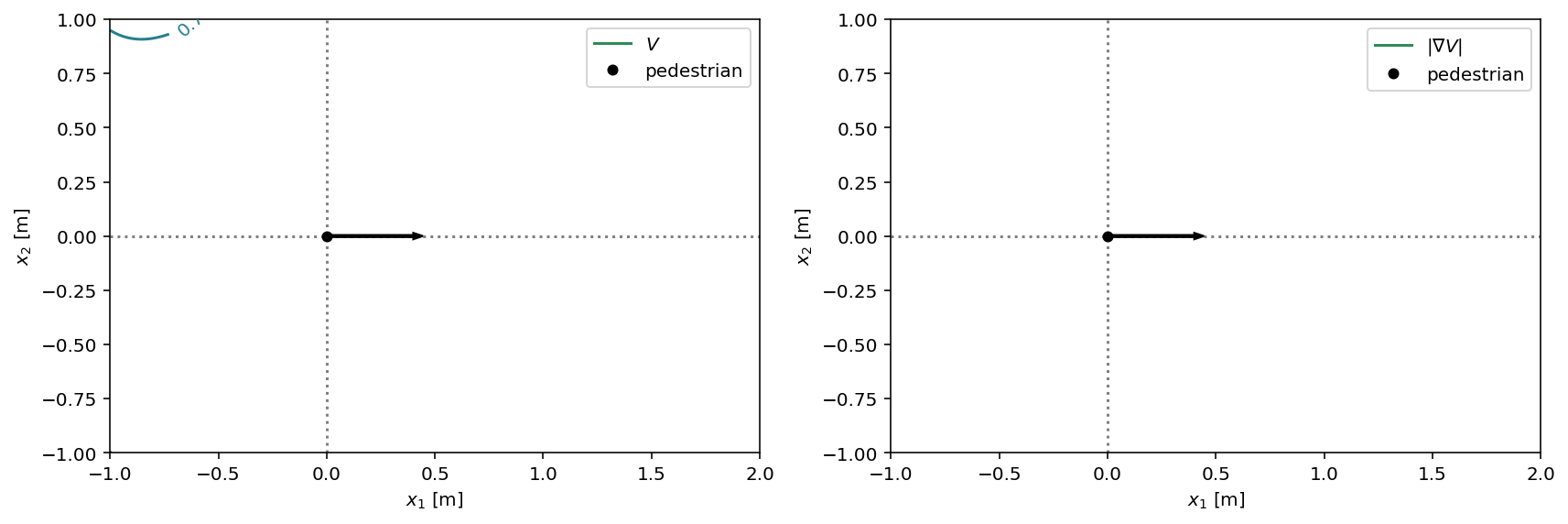
Fourier Features¶

We construct an coordinate-based MLP with Fourier Features [RR+07, TSM+20]. This coordinate-based MLP with the Fourier Feature operator FF is:

(13)¶\[\begin{align} \textrm{MLP}(b, d_{\perp}, d_{\parallel}) &= \textrm{Softplus} \;\; L_{1\times64} \;\; \big[ \textrm{Softplus} \;\; L_{64\times64} \big]^3 \;\; \textrm{Softplus} \;\; L_{64\times192} \;\; \textrm{FF}_{192 \times 3} \;\; (b, d_{\perp}, d_{\parallel}) \end{align}\]

V = socialforce.potentials.PedPedPotentialMLP2D(
    hidden_units=64, n_hidden_layers=2, n_fourier_features=64, tanh_range=3.0, fourier_scale=3.0)
with socialforce.show.canvas(figsize=(12, 6), ncols=2) as (ax1, ax2):
    socialforce.show.potential_2d(V, ax1)
    socialforce.show.potential_2d_grad(V, ax2)

# HIDE OUTPUT
simulator = socialforce.Simulator(ped_ped=V)
opt = torch.optim.SGD(V.parameters(), lr=0.03, momentum=0.9, nesterov=True)
socialforce.Trainer(simulator, opt).loop(10, true_experience)

epoch 1: 0.015041447569032392

epoch 2: 0.009004531869431643

epoch 3: 0.007789137978996948

epoch 4: 0.00705370857701363

epoch 5: 0.006828486191971782

epoch 6: 0.00648589138611507

epoch 7: 0.006311069075588899

epoch 8: 0.0064089279589596045

epoch 9: 0.0059767859865988105

epoch 10: 0.005932234657303206

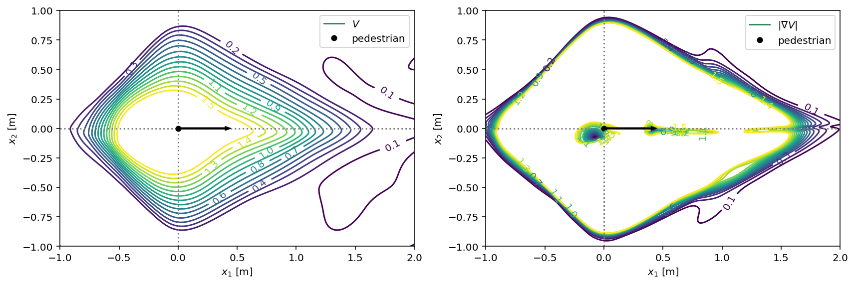
with socialforce.show.canvas(figsize=(12, 6), ncols=2) as (ax1, ax2):
    socialforce.show.potential_2d(V, ax1)
    socialforce.show.potential_2d_grad(V, ax2)

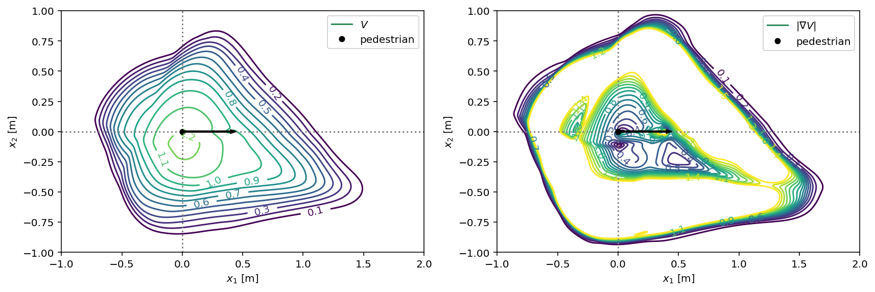
Asymmetric¶

We can redo the above steps with an asymmetric version of the diamond potential. This refines the previous model by a short training on the scenarios generated with the modified potential.

V_asym = socialforce.potentials.PedPedPotentialDiamond(sigma=0.5, asymmetry_angle=-20.0)
with socialforce.show.canvas(figsize=(12, 6), ncols=2) as (ax1, ax2):
    socialforce.show.potential_2d(V_asym, ax1)
    socialforce.show.potential_2d_grad(V_asym, ax2)

circle_asym = socialforce.scenarios.Circle(ped_ped=V_asym)
parallel_overtake_asym = socialforce.scenarios.ParallelOvertake(ped_ped=V_asym, b_center=0.25)
parallel_avoidance_asym = socialforce.scenarios.ParallelAvoidance(ped_ped=V_asym, b_center=-0.25)
scenarios_asym = circle_asym.generate(50) + parallel_overtake_asym.generate(50) + parallel_avoidance_asym.generate(150)
true_experience_asym = socialforce.Trainer.scenes_to_experience(scenarios_asym)

From the perspective of the primary pedestrian:

# HIDE CODE
with socialforce.show.track_canvas() as ax:
    socialforce.show.experience(ax, true_experience_asym)

# HIDE OUTPUT
socialforce.Trainer(simulator, opt).loop(10, true_experience_asym)

epoch 1: 0.009228332611718343

epoch 2: 0.006972365520796904

epoch 3: 0.006454007300254202

epoch 4: 0.006139285584868661

epoch 5: 0.006026841439435587

epoch 6: 0.005688764077679059

epoch 7: 0.005738585170912209

epoch 8: 0.006114561652627816

epoch 9: 0.005619343535467566

epoch 10: 0.005792415339311301

with socialforce.show.canvas(figsize=(12, 6), ncols=2) as (ax1, ax2):
    socialforce.show.potential_2d(V, ax1)
    socialforce.show.potential_2d_grad(V, ax2)

DeepSocialForce