1D
Parametric
We start with the simple case where the potential \(V(b)\) is approximated only by the classical Social Force potential SF:
with its two parameters \(V_0\) and \(\sigma\). Although it is a single-argument function, the argument \(b\) is the semi-minor axis of an ellipse, a 2D object:
as defined in [HM95] with \(\vec{r}_{\alpha\beta} = \vec{r}_{\alpha} - \vec{r}_{\beta}\). We can compare this with \(2b = \sqrt{(p + q)^2 - d^2}\) where the three parameters are the distance to the first focal point \(p\), the distance to the second focal point \(q\) and the distance between the focal points \(d\).
We can visualize this potential in terms of its value and the magnitude of its gradients in the physical coordinates of a pedestrian:
V = socialforce.potentials.PedPedPotential()
with socialforce.show.canvas(figsize=(12, 6), ncols=2) as (ax1, ax2):
    socialforce.show.potential_2d(V, ax1)
    socialforce.show.potential_2d_grad(V, ax2)
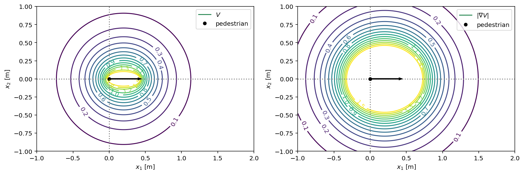
The pedestrian is located in the left focal point of the ellipse and at their current speed can reach the right focal point within one step that is assumed to take \(\Delta t = 0.4s\).
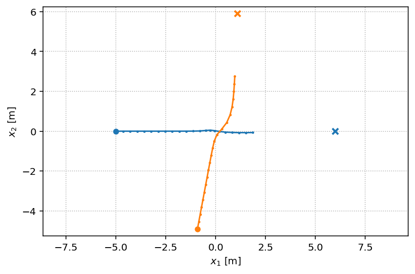
Scenario
We generate a single Circle scenario.
circle = socialforce.scenarios.Circle()
scenarios = circle.generate(1)
true_experience = socialforce.Trainer.scenes_to_experience(scenarios)

with socialforce.show.track_canvas() as ax:
    socialforce.show.states(ax, scenarios[0])
MLP
We infer the parameters of an MLP to approximate the 1D scalar
function \(\textrm{SF}(b)\) above from synthetic observations.
The PedPedPotentialMLP is a two-layer MLP with softplus activations:
which is written in terms of linear and non-linear operators where the Softplus operator applies the softplus function on its input from the right and \(L\) is a linear operator (a matrix) with the subscript indicating the \(\textrm{output features} \times \textrm{input features}\). This two-layer MLP with 5 hidden units has 10 parameters.
V = socialforce.potentials.PedPedPotentialMLP()
initial_state_dict = copy.deepcopy(V.state_dict())
Inference
We use a standard optimizer from PyTorch (SGD).
You can specify a standard PyTorch loss function for the Trainer as well
but here the default of a torch.nn.L1Loss() is used.
# HIDE OUTPUT
simulator = socialforce.Simulator(ped_ped=V)
opt = torch.optim.SGD(V.parameters(), lr=1.0)
socialforce.Trainer(simulator, opt).loop(100, true_experience, log_interval=10)
final_state_dict = copy.deepcopy(V.state_dict())
epoch 10: 0.012704348657280207
epoch 20: 0.011032671725843102
epoch 30: 0.009940878197085112
epoch 40: 0.008118671830743551
epoch 50: 0.004918028542306274
epoch 60: 0.0024081429291982204
epoch 70: 0.001359142188448459
epoch 80: 0.0010096965706907213
epoch 90: 0.0010789994266815484
epoch 100: 0.0010910755081567913
# HIDE CODE
with socialforce.show.canvas(ncols=2, figsize=(10, 4)) as (ax1, ax2):
    socialforce.show.potential_1d_parametric(
        circle.ped_ped, ax1, ax2,
        label=r'true $V_0 e^{-b/\sigma}$', sigma_label=r'true $\sigma$', color='gray')

    V.load_state_dict(initial_state_dict)
    socialforce.show.potential_1d(V, ax1, ax2, label=r'initial MLP($b$)', linestyle='dashed', color='C0')

    V.load_state_dict(final_state_dict)
    socialforce.show.potential_1d(V, ax1, ax2, label=r'MLP($b$)', color='C0')
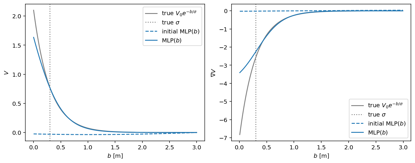
We generated a single synthetic scene with two pedestrians with a parametric potential that was the standard Social Force potential. That parametric potential is shown in gray in the above plot. Then we trained an MLP to infer its parameters. In the above plot, you see the MLP with its initialized random parameters as a dashed line and with its inferred parameters as a solid line. During the training process, the function values of the generating potential were never accessed. Only observed simulation steps were used to train the potential.